602-840-0606
Toll-Free: 800-238-7475
contact@cmyers.com
| Cookie | Duration | Description |
|---|---|---|
| cookielawinfo-checkbox-analytics | 11 months | This cookie is set by GDPR Cookie Consent plugin. The cookie is used to store the user consent for the cookies in the category "Analytics". |
| cookielawinfo-checkbox-functional | 11 months | The cookie is set by GDPR cookie consent to record the user consent for the cookies in the category "Functional". |
| cookielawinfo-checkbox-necessary | 11 months | This cookie is set by GDPR Cookie Consent plugin. The cookies is used to store the user consent for the cookies in the category "Necessary". |
| cookielawinfo-checkbox-others | 11 months | This cookie is set by GDPR Cookie Consent plugin. The cookie is used to store the user consent for the cookies in the category "Other. |
| cookielawinfo-checkbox-performance | 11 months | This cookie is set by GDPR Cookie Consent plugin. The cookie is used to store the user consent for the cookies in the category "Performance". |
| viewed_cookie_policy | 11 months | The cookie is set by the GDPR Cookie Consent plugin and is used to store whether or not user has consented to the use of cookies. It does not store any personal data. |
c. myers live – Key Components of Thinking Critically – Takeaways from Senior Leaders
Featured, Strategic Leadership Development, Strategic Planning PodcastsWith the financial services industry changing faster than ever, it is essential for teams to practice critical thinking to accelerate their depth of thinking and execution of the things that really matter. In this c. myers live, we will reflect on some takeaways from our Critical Thinking Workshop that participants found valuable for implementation within their own organization.
For more information about our upcoming Critical Thinking Workshop in December, please click here.
About the Hosts:
Adam Johnson
Learn more about Adam
Brian McHenry
Learn more about Brian
Other ways to listen to c. myers live:
Static and Dynamic Methodologies – Critical ALM Modeling Issues That Can’t Be Ignored
ALM, Featured, Financial Planning, Interest Rate Risk Blog Posts7 minute read – As rates have increased materially, and liquidity pressure continues to build, leaders will continue to be faced with high-impact decisions that can have longer term consequences. Reliable and timely financial decision-information is a huge component of a successful decision-making process.
This blog on Static Balance Sheet Analysis (sometimes referred to as Static NII or Net Interest Income) and Dynamic Simulations is part of a series addressing critical ALM modeling issues.
Static Balance Sheet Analysis, by definition, assumes that the balance sheet structure never changes, even if rates change. The static methodology was developed prior to advanced computing power. Unfortunately, it has remained pervasive in modern risk analysis. This simplified methodology is particularly dangerous and misleading in the rate environments decision-makers are facing today, as it can understate risk. For example, many institutions’ ability to attract funding is shrinking and the mix of funding is changing to higher cost sources. This is completely ignored in a Static Balance Sheet simulation.
Problem: Static reflects none of the potential liquidity pressure that has historically occurred when rates rise, ignoring the resulting change in funding mix and its impact on the cost of funds.
Solution 1: First and foremost, make sure the limitations of the Static Balance Sheet Analysis are clear to other decision-makers to avoid unpleasant surprises.
Solution 2: Incorporate a methodology that automatically changes the mix of deposits as rates change.
Problem: There are no fixes to the Static Balance Sheet methodology that also preserve the true definition of static. However, there are some work-arounds if your modeling capabilities or policies are limited to Static Balance Sheet Analysis.
Solution: Create a non-maturity deposit category to represent the non-maturity deposits that could shift to CDs as rate advantages develop. Move some of the starting funds into that account and have it reprice to your new CD rates. (Keep in mind your average balance per account pressure along with the consumer’s advantage to move to CDs)
There are also problems with Dynamic Simulations, many of which are solvable. Here are just a few considerations.
Problem: Similar to the issue with Static Balance Sheet Analysis, many Dynamic Simulation models do not incorporate decay rates when quantifying risks to earnings and capital.
Keeping the same future balance, regardless of market rates, doesn’t appropriately address the exposure and can understate the volatility. It misses the risk that the funding mix can change and the resulting impact to the cost of funds.
Ask Yourself: As discussed in previous blogs, why is it standard practice to apply decay assumptions when doing EVE/NEV and yet this practice is ignored in typical Static and Dynamic Balance Sheet Analysis?
Solution: You will need to make manual adjustments to represent the potential reductions in balances on the lower-priced products and the shift to higher-priced products, if appropriate. While it is not difficult to make this assumption for one environment, most models do not have the ability for the non-maturity balance to automatically change for each rate environment simulated.
Problem: Assumptions regarding new business can hide risks that currently exist or introduce risks that don’t exist. This muddies the waters for decision-makers and can lead to overconfidence in the risk position or unnecessary de-risking.
Solution: Run simulations that isolate existing risk/return, focusing on the potential profit and capital impact in the current structure. A benefit of this is to see the potential timing of risk and what it may take to offset the risk if exposure is too high. This will help decision-makers have more clarity as to the sources of risks and returns before deciding the best course of action.
Problem: Focusing on the relative rate environment and consistency in assumptions is overrated. The rate environment has changed drastically in recent months and assumptions assigned to current and up/down rate environments deserve a thorough review. These types of assumptions can heavily influence the results of risks to earnings, capital, and EVE/NEV.
Solution: Dig deep into your decay rate assumptions to ensure that the actual current rate environment, which changes over time, is being considered. This is a hard, yet critically needed, shift in ALM modeling mindset. This is only one of many examples regarding assumptions that need to be reviewed. This is addressed in detail in our blog on decay rates.
As we said in the beginning, reliable financial decision-information is critical to thriving in this type of environment.
We run thousands of risks to earnings, capital, and EVE/NEV simulations and what-ifs each year, so we understand the considerations facing finance teams today – this blog just scratches the surface. We know that timing is critical and finance teams need to move fast. Please feel free to call us if you have questions on the information provided in this blog.
You may also be interested in:
c. myers live – Pricing and Withdrawals: Critical ALM Issues
ALM, Featured, Financial Planning PodcastsIn this episode of c. myers live, we discuss critical ALM modeling issues that impact decision-making, in this challenging environment. We recently wrote a blog about a specific ALM modeling issue, with respect to decay rates. This podcast builds on this critical conversation and works to simplify a complex set of financial concepts through discussion.
The show notes below go hand-in-hand with this episode of c. myers live.
We’re delving into capturing consumer behaviors surrounding deposits with modeling assumptions to produce better decision information.
The Changing Environment
Consider what happened in 2021, when total deposit balances and average account balances increased for most institutions and account types. Contrast that with what is happening now that market rates are higher.
Think about it from the consumer’s perspective and the concept of the advantage to the consumer to move their money to another product or institution:
This illustrates that consumer behavior is different when the advantage increases (18% decline in balances versus 0%), yet the following example of decay rates is typical of what is found in many models and does not reflect any change in behavior between 2021 and 2022.
If your model looks roughly like these two simple examples, then it would assume 10% withdrawals in the starting position and 20% in +200, even though current rates are a lot higher and provide a much larger reason to move.
Linking Withdrawals/Decays to the Advantage
Remember that the advantage in December 2021 was 0.85% and for December 2022 it was 3.90%. A single table like this, for the rate environment in December 2021, would result in an assumption of 0% since the advantage is less than 1%. Then in December 2022, since the advantage to move money increased, the table would automatically shift the “Base” situation to be 20% withdrawals. Note, a table design like this connects the rate paid in each environment and the alternative for the customer to move their funds. The shift of +200 or +300 in December 2022 would automatically show more risk of liquidity pressure (cost of liquidity) than a +200 or +300 would have shown in 2021.
What could you do if your model doesn’t have this ability? It is not ideal, but you could keep a side table storing your assumptions from an advantage perspective, since that can be a major motivator for moving deposits. Then as the environment changes, update the assumptions in the model to mimic the table you have on the side. For example:
Don’t focus on the specific numbers in the examples, as the numbers vary by institution and account type.
Note that to simplify the example, we only showed one deposit type. Most institutions have many deposit types. Additionally, as mentioned in the podcast, we recommend breaking material deposit types into balance tiers that may have different behaviors.
The Financial Impact of Decays/Withdrawals
Keep in mind, there are many strategic implications to consider with deposit pricing, including your desired brand, target market, value proposition, competitive environment, and long-term goals, to name a few. It is also important to understand the math of what the potential impact could be and connect it to the strategy to help understand trade-offs and alternatives.
In the podcast, Rob and Sally gave an example of a category that has $1 Billion in deposits. To make the numbers even simpler, the tables below are for a deposit category that has $100 Million in deposits.
If decays/withdrawals are not incorporated in earnings impact: Typical Static Balance Sheet
If current experience is 10% decline, and the simulation assumes the decline does not change when paying higher rates:
If current experience is 10% decline, and you think paying 1% would stop the outflow, but paying 0.30% would not change behavior: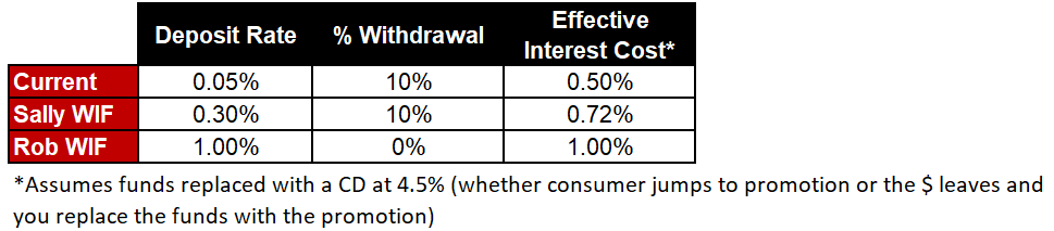
If current experience is 30% decline, and the simulation assumes the decline does not change when paying higher rates:
If current experience is 30% decline, and you think paying 1% would stop the outflow, and paying 0.30% would slow some of the outflow:
Any decision to change non-maturity deposit rates on a category that has material balance is a big decision, as it will have an immediate impact on earnings. As mentioned earlier, there are strategic, philosophical, and financial reasons to consider when evaluating a change. The key is to ensure that the financial impact being modeled is representing the expectations or concerns that decision-makers are working to address.
Modeling Decay/Withdrawal Rates in the Income Simulation
Many models do not apply decay/withdrawal assumptions to the income simulations; they only use those assumptions for economic value results. If this is the case, then additional work should be done to model the earnings impact of withdrawals when modeling pricing changes.
Without decay/withdrawal assumptions, any increase in deposit rates will cost the institution the amount of increase without any potential for an offsetting behavior, such as less movement to higher priced funding sources.
If you’re wondering if the extra work is worth it, think about it this way. If you truly believed that the consumer with funds in deposits doesn’t care about rate and won’t ever change their behavior, then there wouldn’t be a reason to pay anything on the account and it would be better to use that earnings impact on another area that could increase your value proposition.
About the Hosts:
Sally Myers
Learn more about Sally
Rob Johnson
Rob, President and one of five c. myers owners, has been instrumental in delivering on the vision of enabling leadership teams to have relevant and reliable financial decision-information at their fingertips, so that they can accelerate their strategic impact in providing value to their markets. Clients find the speed of the decision-information, whether at the enterprise level or drilling into what is driving profitability at a category level, combined with Rob’s quick mind and critical thinking, to be invaluable.
Learn more about Rob
Other ways to listen to c. myers live:
c. myers live – Are You Getting the Strategic Progress That You Want?
Featured, Process Improvement, Strategic Implementation, Strategic Planning Blog PostsAs we enter a new year with strategic plans concluded, it is now time to hit the ground running on the list of key projects that will move the strategy forward. After receiving great feedback on this c. myers live we posted last year, we want to remind executives of a few ways to keep planning and implementation aligned with your strategic goals and continue utilizing the planning process to make sure your institution is making strategic strides in the right direction now and throughout the year.
About the Hosts:
Brian McHenry
Learn more about Brian
Dan Myers
Learn more about Dan
Other ways to listen to c. myers live:
Decay Rates – A Critical ALM Modeling Issue That Can’t Be Ignored
ALM, Featured, Financial Planning Blog Posts5 minute read – As rates have increased materially, and liquidity pressure continues to build, leaders will continue to be faced with high-impact decisions that can have longer-term consequences. Reliable and timely financial decision-information is a huge component of a successful decision-making process.
This blog on decay rates is the first in a series addressing critical ALM modeling issues. There is a lot of information here, so pull it up on the big screen for a better view.
Problem: When conducting EVE/NEV simulations, the focus on the relative rate environment is overrated. This focus can result in a misinterpretation of how assumptions are being applied, and heavily influences the results.
Solution: Dig deep into your decay rate assumptions to ensure that the actual current rate environment, which changes over time, is being considered. This is a hard, yet critically needed, shift in ALM modeling mindset and is only one of many examples regarding assumptions that need to be reviewed.
This concept can be a little harder to visualize so we have added some tables to help. Tables A and B are simple examples of the format we often see when doing model validations.
Are the assumptions consistent?
No. While on the surface they look the same, if you dig deeper, they are not. Keep in mind that as of December 2021, the current 3-Month Treasury was about 0.1%. At the end of December 2022, it was around 4.40%. This fact is easy to miss because there is no statement of what the current environment actually is.
To illustrate why the actual rates do matter, we added a row of information to Tables C and D that most models don’t address. The inconsistency becomes much clearer.
Focus on the highlighted lines to see inconsistencies in the assumptions.
Just a few considerations as you review your assumptions for reasonableness:
Problem: Many decision-makers think that the decay tables used for EVE/NEV apply when simulating risks to earnings and capital. Unfortunately, many models do not link the decay rates when simulating risks to earnings and capital, which can understate the risk. This approach is essentially saying that the consumer does not care what rates they are paid. This does not make sense.
Ask yourself: What is the rationale to incorporate decay rate assumptions when doing EVE/NEV simulations, and not when simulating risks to earnings and capital? Remember, liquidity has become a bigger topic in many C-Suite and board discussions. It is important to clarify for stakeholders which ALM results that you review incorporate the risk of withdrawals/decays and which results do not.
As we said in the beginning, reliable financial decision-information is critical to thriving in this type of environment. We run thousands of risks to earnings, capital, and EVE/NEV simulations and what-ifs each year.
This blog just scratches the surface of considerations facing finance teams today. Stay tuned for more tips on providing reliable financial decision-information.
We understand timing is critical and finance teams need to move fast. Please feel free to call us if you have questions on the information provided in this blog and/or just can’t wait for our upcoming blogs.
You may also be interested in: